Choosing the Right Regression

What each family solves and when to use it

Knowing the names of regression algorithms is useful. Knowing which question each one answers is what makes that knowledge usable.

Consider a payment platform. You might want to predict the amount of the next transaction, the probability that it is fraudulent, the number of failed payments next hour, or how long a merchant will remain active. These questions involve the same business and may use similar inputs. They require different treatment of the outcome.

A sensible choice starts with the target, the decision the prediction will support, and how the observations were collected. Model complexity comes later.

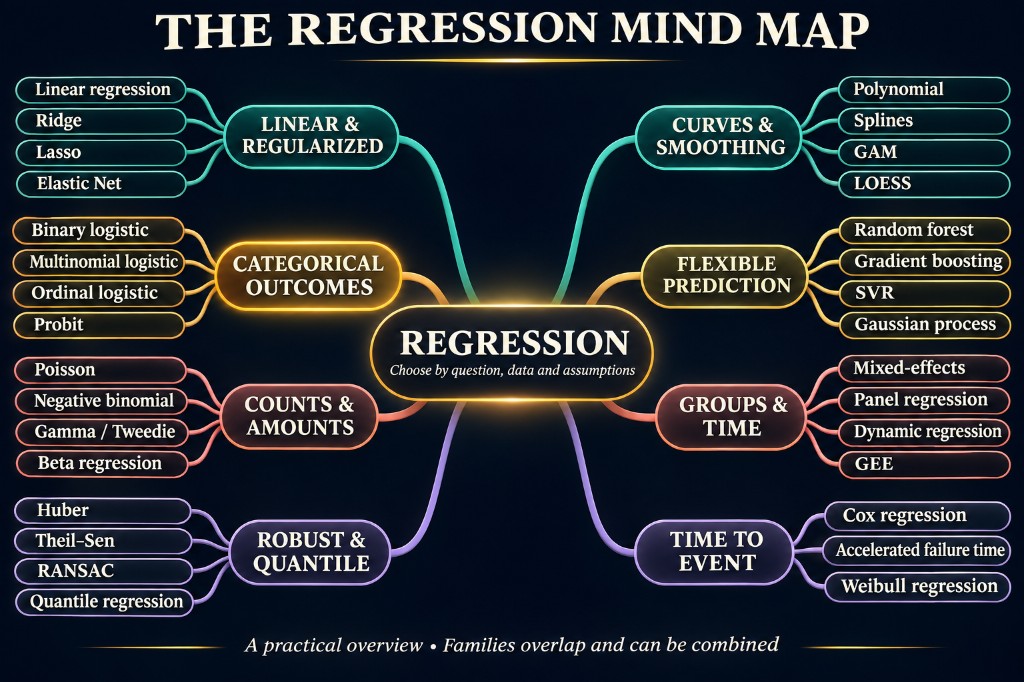
There is no final catalogue of every regression. Some names describe the mathematical relationship, some describe the outcome distribution, and others describe how a model is fitted. These choices can be combined. A model can be a regularized logistic regression with spline features and hierarchical effects at the same time.

The families below provide a practical map, followed by a selection process you can apply to a real project.

The regression mind map: choose by question, data and assumptions

First decide what you want the model to estimate

For a numerical outcome, “predict the value” leaves an important question unanswered: which aspect of the outcome?

For delivery time, the conditional mean answers how long delivery takes on average for orders with given characteristics. The median describes the middle of that distribution. The 95th percentile describes a duration below which roughly 95% of comparable deliveries should fall, if the model is well calibrated.

Those are different products. A staffing plan might need expected demand. A delivery promise might need an upper quantile. Neither is automatically the right answer for the other decision.

Also distinguish three goals:

Prediction: What is likely to happen for a new observation?
Association and explanation: How does the outcome vary with the observed inputs, under a specified model?
Causal estimation: What would change if we intervened?

A regression coefficient does not, by itself, establish causation. A model can predict purchases accurately from browsing history without telling us what would happen if we changed the website. Causal questions require assumptions and a defensible study design in addition to an estimator.

Linear regression: an interpretable numerical baseline

Simple linear regression uses one predictor. Multiple linear regression uses several. Both model a numerical outcome through a weighted combination of features.

For example, a first model of cloud expenditure might combine request volume, storage usage, and active customer count. Its coefficients describe associations with expected expenditure, conditional on the other included features.

Use it when: you need an understandable baseline and an additive relationship is a reasonable starting approximation.

Watch for: curvature, interactions, unstable coefficients, and structured residuals. Residuals are the differences between observed values and fitted predictions.

Ordinary least squares, or OLS, fits the model by minimizing squared residuals. Weighted least squares, or WLS, can account for observations with different error variances through suitable weights. Generalized least squares, or GLS, handles a specified error covariance structure. These are estimation approaches, not three unrelated prediction tasks.¹

“Linear” refers to the coefficients. A model containing squared inputs or interaction terms can still be linear in its parameters.

Polynomial, interaction, and segmented regression

An extra hour of training may matter much more for a beginner than for someone who has already completed 200 hours. A single constant slope may miss that pattern.

Polynomial regression adds powers such as x². Interaction terms allow the association with one feature to depend on another. Segmented regression uses different relationships in different regions, sometimes with continuity at the boundaries.

For example, request volume may have a modest relationship with latency until a system reaches a capacity threshold. After that threshold, latency may rise sharply. A segmented model can express this more naturally than one global line.

Use them when: you have a plausible reason for curvature, a threshold, or a conditional effect.

Watch for: excessive flexibility and extrapolation. A high-degree polynomial can fit observed data closely and produce implausible values just outside the observed range. Adding more terms also increases the need for validation and, often, regularization.

Ridge, Lasso, and Elastic Net

Many predictors can describe nearly the same underlying signal. Customer activity might appear as sessions, clicks, visits, and time spent. A model can struggle to assign stable individual coefficients to these overlapping measurements.

Method	What it changes	When it is useful
Ridge	Adds an L2 penalty that shrinks coefficients	Many correlated inputs may all contain useful signal
Lasso	Adds an L1 penalty that can set coefficients to zero	A sparse predictive model is desirable
Elastic Net	Combines L1 and L2 penalties	Correlated inputs and sparsity are both relevant

Choose penalty strength through validation. Feature scaling matters because the penalty acts on coefficient magnitudes. Lasso selection is not proof that retained variables are causal or uniquely important; correlated variables can substitute for one another.²

More specialized variants include Group Lasso, which selects groups of features, and Fused Lasso, which encourages related coefficients to be similar. The useful question is what structure the penalty should encourage.

Logistic regression: estimating probabilities for categories

Logistic regression deserves its own place because its name often causes confusion. It is usually used for classification, even though it belongs to the broader statistical regression tradition.

Binary logistic regression estimates a probability between zero and one. A classification decision then applies a threshold to that probability. Multinomial logistic regression extends the approach to several unordered classes. Regularization can be applied here too.³

For a payment platform, the target might be whether a transaction is fraudulent. The model could return an estimated probability of 0.08. Whether that triggers a review depends on the cost of missed fraud, the cost of unnecessary reviews, and the review team's capacity. The threshold is a decision rule, not an unavoidable property of the model.

Use it when: the target is categorical and you want a relatively transparent probability model.

Watch for: probability calibration, class imbalance, and nonlinear effects. Logistic regression does not require probability itself to change linearly with a predictor; its standard formulation is linear on the log-odds scale.

For ordered outcomes such as low, medium, and high satisfaction, consider ordinal logistic regression. A common form assumes proportional odds, which should be checked. Probit regression is another categorical-outcome approach, using a different link function.

Encoding classes as 0, 1, and 2 does not automatically make ordinary numerical regression appropriate. That encoding can impose distances between categories that have no defensible meaning.

Count regression: predicting how many events occur

Counts include support tickets, failed payments, defects, and purchases. They are nonnegative integers, although the predicted expected count can be fractional.

Poisson regression is a common starting point. It assumes equality of conditional mean and variance. Negative binomial regression allows a particular form of overdispersion: conditional variance larger than the mean.⁴

For example, incidents may cluster on difficult operational days. If variability remains much larger than a Poisson model allows after accounting for the predictors, a negative binomial model becomes a candidate.

Use them when: the outcome is an event count within a defined observation window.

Watch for: exposure. Five incidents over one hour and five over one month describe different rates. In a log-link count model, an exposure offset can account for different observation durations or opportunities.

Zero-inflated models add a separate source of zeros. Hurdle models separate zero versus positive outcomes, then model positive counts. Both have Poisson and negative binomial variants.⁵

Many zeros alone do not justify either approach. Low expected counts naturally generate zeros. Ask whether the underlying process supports a separate zero mechanism, then compare the models.

Positive amounts and proportions

Some quantities cannot be negative. Others must remain within a fixed interval. A model should reflect these constraints where they matter.

Gamma regression, often with a log link, is a candidate for strictly positive, right-skewed amounts. Inverse Gaussian regression provides another positive-outcome family with a different mean–variance relationship. A Tweedie model with power between one and two can represent a point mass at zero alongside positive continuous amounts.⁴

For example, daily customer expenditure may contain many exact zeros and occasional large purchases. Gamma alone cannot represent those zeros. A suitable Tweedie model or a two-part model can be more natural.

Beta regression models continuous proportions strictly between zero and one, with parameters governing their mean and precision. It is useful for outcomes such as a continuously measured utilization fraction. Exact zeros or ones require another approach or an appropriate extension.⁶

The origin of a proportion matters. If a conversion rate comes from 12 purchases among 100 visitors, a binomial model can preserve the denominator. A 12% rate based on 100 visitors carries different information from 12% based on 100,000.

Use these families when: the range and variability of the outcome are central to the problem.

Watch for: choosing a distribution from the raw histogram alone. Regression describes outcomes conditional on the predictors, so assess the fitted model as well.

Robust regression

Squared-error fitting can be pulled strongly by large residuals. Robust regression changes how those residuals influence estimation.

Huber regression uses a loss that is quadratic near zero and linear for sufficiently large residuals. Other robust M-estimators use different influence or weighting functions.⁷

Theil–Sen uses a median-based approach. RANSAC repeatedly fits candidate subsets to seek a model supported by an inlier set. Their definitions of robustness differ; no method is universally resistant to every kind of contamination.

Use robust methods when: measurement errors or contamination could distort an otherwise useful relationship.

Watch for: treating meaningful extremes as bad data. An unusually expensive outage may be exactly what the model needs to learn about. Investigate whether an outlier is an error, a rare legitimate event, or evidence of another operating regime before reducing its influence.

Robust fitting also differs from robust standard errors. The latter adjust uncertainty estimates without necessarily changing the fitted coefficients.

Quantile regression

Quantile regression estimates a chosen conditional quantile. At 0.5 it targets the conditional median; at 0.9 it targets the conditional 90th percentile. Linear quantile regression commonly uses pinball loss, and some implementations also apply regularization.⁸

Suppose two delivery services both average two days. One is consistently close to two days; the other alternates between very fast and very slow deliveries. Their averages do not reveal the difference that matters to a customer receiving a delivery promise.

Use it when: you need upper or lower outcome boundaries, asymmetric planning, or a view of how predictors affect different parts of a distribution.

Examples include capacity planning, delivery commitments, and estimating high latency rather than average latency.

Watch for: sparse data in extreme tails and crossing predictions when quantiles are fitted separately. An estimated 95th percentile is not a guarantee for an individual case. Check how often observed outcomes actually fall below it, including within relevant subgroups.

Splines and GAMs

Splines represent curves using connected basis functions. A generalized additive model, or GAM, combines smooth effects of predictors and can use different outcome families and link functions. Smoothness penalties control complexity.⁹

For an energy model, temperature might have a U-shaped association with demand: cooling at one extreme and heating at the other. A GAM can represent that shape without forcing a straight line or one high-degree global polynomial.

Use them when: effects are nonlinear but you still want to inspect individual modeled relationships.

Watch for: interactions. A basic additive structure does not automatically capture a relationship where the effect of temperature depends on building type. Such structure must be included appropriately.

LOESS and LOWESS provide local smoothing alternatives, especially useful for exploration. A smooth curve is evidence of a fitted pattern, not proof of a causal mechanism.

Trees, forests, and boosting

A regression tree divides the feature space into regions. Random forests aggregate randomized trees. Extra Trees introduce further randomness into splitting. Gradient boosting adds models sequentially to improve an objective. XGBoost, LightGBM, and CatBoost are implementations of boosting methods, rather than separate kinds of regression target.¹⁰

Use these approaches when: you suspect substantial nonlinearities and interactions in tabular data and predictive performance is a central goal.

For example, delivery time may depend on a combination of warehouse, region, order size, and time of day. Trees can discover useful conditional splits without manually specifying every interaction.

Watch for: overfitting, leakage, and weak extrapolation. Conventional regression trees and forests do not learn a continuing linear trend beyond their observed ranges. Feature importance also does not establish causality.

These methods should earn their additional complexity through validation against a credible baseline.

SVR, Gaussian processes, nearest neighbours, and neural networks

These approaches offer different ways to model complex functions.

Method	What it does	When to consider it	Main limitation
Support vector regression (SVR)	Fits a function with a tolerance region; kernels allow nonlinear relationships	Small or medium datasets where a suitable kernel captures the structure	Scaling, tuning, and computational cost
Gaussian process regression	Defines a distribution over functions and produces model-based predictive uncertainty	Expensive experiments, surrogate models, and relatively small datasets	Exact inference scales poorly; uncertainty depends on assumptions
k-nearest neighbours regression	Predicts from nearby observations	A meaningful distance measure and informative local similarity	High dimensions and irrelevant features weaken neighbourhoods
Neural network regression	Learns a flexible mapping from inputs to numerical outputs	Rich inputs, complex structures, and enough relevant training data	Tuning, data needs, and harder interpretation

SVR and Gaussian processes depend strongly on kernel choice. A kernel expresses what kinds of similarities or function shapes the model considers plausible. Gaussian process uncertainty should still be checked against held-out outcomes.¹¹¹²

For a dataset with a few hundred rows and ten ordinary business variables, a neural network should demonstrate a benefit over simpler candidates before it becomes the default.

Grouped observations: mixed-effects, hierarchical models, and GEE

Repeated observations from the same person, merchant, school, or branch are not automatically independent.

Mixed-effects models combine population-level effects with group-specific variation, such as random intercepts or slopes. Hierarchical models can partially pool information between groups.¹³

For example, a delivery-time model may need to represent persistent warehouse differences while learning shared associations with order size. Estimating each warehouse completely separately can be unstable for small warehouses; ignoring warehouses entirely loses structure.

GEE, or generalized estimating equations, provides a different approach for estimating population-average relationships with clustered or repeated observations.¹⁴

Use these approaches when: observations are clustered and that dependence affects estimation, uncertainty, or the intended predictions.

Watch for: confusing the goal of predicting another observation from a known group with predicting for a completely new group. Those deployment situations require different validation designs.

Panel fixed-effects and random-effects models address related questions for repeated observations across entities and time. Their assumptions, especially about relationships between entity effects and predictors, affect interpretation.

Time-to-event regression

Suppose you study customer retention for one year. Some customers leave; others remain active at the end. For those still active, you know their retention time exceeds the observed follow-up. You do not know their final retention duration.

That is right censoring. Survival models are designed to use this information rather than treating the end of observation as the event time.

Cox proportional hazards regression relates predictors to the hazard, an instantaneous event rate among those still at risk. A common assumption is that hazard ratios remain constant over time. Accelerated failure time models instead describe how predictors stretch or shorten event times. Parametric alternatives include Weibull, log-normal, and log-logistic models.¹⁵

Use them when: the question is how long until failure, churn, completion, or another event, especially when follow-up is incomplete.

Watch for: the censoring mechanism and model assumptions. Dropping customers who have not yet left can systematically distort the question you are answering.

Specialized structures

Some problems require more than choosing a familiar loss function.

Situation	Candidate approach	Why it matters
Past outcomes help predict future outcomes	Autoregression or dynamic regression	Accounts for temporal structure
Predictors explain part of a time series, but residuals remain correlated	Regression with ARIMA errors	Models remaining serial dependence
Values are recorded only up to a reporting limit	Censored regression, such as an appropriate Tobit model	Observed limits are not the underlying values
Observations outside a range never enter the dataset	Truncated regression	The sampling process changes the observed distribution
Both x and y contain measurement error	Errors-in-variables or Deming regression	Ordinary fitting may distort slopes
Outcomes depend on neighbouring locations	Spatial regression	Accounts for spatial dependence
Domain knowledge requires a monotonic response	Isotonic regression or a monotonic constrained model	Encodes a defensible shape constraint
Several numerical outcomes are modeled together	Multivariate or multi-output regression	Can represent or exploit shared structure

Bayesian regression is another cross-cutting framework: it combines a likelihood with prior distributions to estimate a posterior. It can be linear, logistic, hierarchical, or nonlinear. It is useful when prior information and uncertainty matter, but its conclusions depend on the prior and likelihood assumptions.

Instrumental-variable regression belongs to a different decision context: addressing endogeneity under demanding instrument-validity assumptions. It is not a generic technique for improving predictive accuracy.

A practical first-choice table

Treat these as starting candidates, not automatic winners.

Your question or data characteristic	Start by considering	Check before committing
What numerical value should I expect?	Linear regression or Ridge	Shape, residuals, and held-out error
Which of many related inputs should I retain?	Lasso or Elastic Net	Selection stability and validation
What is the probability of an event?	Logistic regression	Calibration and decision thresholds
Which ordered category is likely?	Ordinal regression	Whether the ordinal assumptions fit
How many events occur?	Poisson or negative binomial	Exposure and conditional dispersion
Why are there zeros and positive outcomes?	Hurdle or zero-inflated model	Whether separate mechanisms are plausible
What positive amount is expected?	Gamma or an appropriate transformed model	Zeros, tail behaviour, and retransformation
What continuous fraction is expected?	Beta regression	Endpoints and how the fraction was formed
What upper outcome boundary should I plan for?	Quantile regression	Coverage and tail sample size
Are smooth nonlinear effects important?	Splines or GAM	Smoothness and interactions
Are complex tabular interactions important?	Boosted trees or random forest	Leakage, stability, and extrapolation
Are observations grouped?	Mixed-effects models or GEE	Within-group dependence and prediction goal
How long until an event?	Survival regression	Censoring and event-time assumptions
Will the model predict future periods?	Dynamic regression or another temporal model	Chronological validation and feature availability

How to decide whether your choice works

Define the target precisely. “Predict churn” could mean leaving in the next 30 days, leaving at any point, or time until departure. Those definitions change the model, labels, and evaluation.

Build a simple baseline. Compare against a mean, median, historical rate, or seasonal forecast as appropriate. Then try a simple model suited to the target. Complexity should solve an observed limitation.

Match the split to deployment. Random splits can suit independent observations. Future prediction calls for chronological evaluation. Generalization to unseen customers or branches calls for appropriate group separation. Fit preprocessing within training folds, including scaling, imputation, and feature selection.¹⁶

Choose metrics for the decision. MAE measures average absolute error; RMSE gives more emphasis to large errors. Pinball loss evaluates quantile predictions. For probabilities, consider log loss, Brier score, and calibration. Classification thresholds also require decision-oriented measures such as precision and recall. R² alone is insufficient.¹⁷

Inspect failure patterns. Does the model consistently underpredict large orders? Fail for a particular warehouse? Become overconfident during busy periods? A good overall average can hide an operationally important weakness.

Separate fit assumptions from inference assumptions. Non-normal raw inputs do not rule out linear regression. Normality assumptions often concern errors and particular inference procedures. Unequal error variance does not automatically require abandoning a useful mean model; it may require different uncertainty estimation or an appropriate variance model.

Check extrapolation explicitly. If training data contain no more than 10,000 requests per minute, predictions at 100,000 are an additional claim. A smooth curve does not supply evidence for that claim.

Revisit the model when the process changes. A pricing change, a new customer population, or a redesigned payment flow can alter relationships. Validation from the old process may no longer represent future performance.

One business problem, several valid models

Imagine a company asking for an AI model to improve customer retention. Before opening a model library, clarify the operational decision.

To estimate who will leave within 30 days, start with a binary probability model such as logistic regression.
To estimate when customers will leave, consider survival regression and retain censored observations.
To estimate next month's customer spending, examine whether the outcome needs a positive-only or zero-plus-positive model.
To estimate how many support tickets a customer will raise, consider count regression and exposure.
To estimate a high percentile of response time, consider quantile regression.
To estimate the effect of offering a retention discount, define a causal study; predictive churn accuracy does not answer that question.

The same business objective can therefore lead to several defensible models. The selection becomes clearer when the outcome, observation process, and decision are explicit.

Before choosing an algorithm, write one sentence: “For this population, using information available at this moment, I need to estimate this outcome so that we can make this decision.” That sentence will eliminate more unsuitable models than an alphabetical catalogue ever could.

Building a Reliable ML Model — validation, leakage, and metrics before algorithm shopping
ML Algorithms — broader algorithm landscape
ARIMA — time series when specialized structures apply
SHAP — explaining flexible models after you choose them

Technical references

The examples and selection workflow are illustrative synthesis. The following primary documentation provides technical detail for the model families and evaluation methods discussed.